matplotlib & ipympl#
ipympl (the name comes from IPython - MatPlotLib) is the modern way to display matplotlib outputs under IPython / Jupyter
it adds an interactive layer to a plot, that lets you “dive in” the data
in addition, it is also compatible with
ipywidgetsfor adding interactivity of your own (i.e. the ability to change parameters)
a very moving target
over the years, the way to build interactive or animated figures over matplotlib has gone through considerable changes
as compared for example with the time where one could use interact()
hopefully this will now settle, but be wary that the current notebook was written in June 2024, and make sure to check it is still current before using it
executive summary#
not under jupyter book#
at this point, this sort of figures won’t render well under jupyter book, meaning if you read this as a static HTML document, you won’t see the figures
in that case, you are encouraged to download this notebook and run it locally on your computer
requirements#
ipympl requires a separate installation with - wait for it
pip install ipympl
operating mode#
you use it in a notebook in a pretty straightforward way
it is what’s called a matplotlib backend, to you turn it on using the %matplotlib magic
# I recommend to use this form to enable ipympl

%matplotlib ipympl
%matplotlib widget
the docs say that you can also use instead
%matplotlib widget
which works too; however my daily practice is to use the %matplotlib ipympl form because
it more clearly relates to the pip requirement
it tended to work better under vs-code at the time where I tried
reload your kernel#
it is important that the %matplotlib magic appears before you draw any figure
if you find yourself in a situation where you have done a figure with the the default (inline) backend, and you want to switch to ipympl afterwards, then you need to restart your kernel !
some examples#
the examples below are essentially copied as-is right from the doc here https://matplotlib.org/ipympl/examples/full-example.html
go to that page for more details
in particular regarding the use of ion() / ioff()
another useful page
this page here might turn out useful too for learning about ipywidgets https://kapernikov.com/ipywidgets-with-matplotlib/
the figure is natively interactive#
first, let’s see the native interactive tools - in the code it is named the toolbar
import matplotlib.pyplot as plt
import numpy as np
# Testing matplotlib interactions with a simple plot
fig = plt.figure(figsize=(8, 4))
plt.plot(np.sin(np.linspace(0, 20, 100)));
at that point, your figure is interactive:
notice the gray triangle in the lower right corner: you can resize it
hover your mouse on the figure, and you’ll see the toolbar show up; with it you can
select the zoom tool (a square), and then select a region to zoom in
select the home tool, the figure steps back to the oginal vantage point
hover the mouse on the toolbar buttons to get a grip of what they do
now quickly, here are a few things you could do programatically with this toolbar
# Always hide the toolbar
fig.canvas.toolbar_visible = False

# Put it back to its default|
fig.canvas.toolbar_visible = 'fade-in-fade-out'

# Change the toolbar position
fig.canvas.toolbar_position = 'top'

# Hide the Figure name at the top of the figure
fig.canvas.header_visible = False

# Hide the footer
fig.canvas.footer_visible = False

# Disable the resizing feature
fig.canvas.resizable = False

# back on
fig.canvas.toolbar_visible = True
# a funny feature is, you can 'duplicate' the figure, they will both update in sync !

display(fig.canvas)
changing a line plot with a slider#
here’s now a more interesting example, where we create a slider to see how an external parameter impacts the figure
plt.ioff()
again the upstream page https://matplotlib.org/ipympl/examples/full-example.html has more - rather gory - details about using or not interactivity with plt.ion()/plt.ioff()
observe the following:
this no longer uses the
interact()function, that one would have used to achieve this a few years backinstead, thanks to the
slider.observe()call, a change to the slider triggers a call toupdate_lines()which in turn does an ‘in place’ change of the figure, by locating the curve to modify with
lines[0].set_data()
# When using the `widget` backend from ipympl,
# fig.canvas is a proper Jupyter interactive widget, which can be embedded in
# an ipywidgets layout. See https://ipywidgets.readthedocs.io/en/stable/examples/Layout%20Templates.html

# One can bound figure attributes to other widget values.
from ipywidgets import AppLayout, FloatSlider

plt.ioff()

slider = FloatSlider(
    orientation='horizontal',
    description='Factor:',
    value=1.0,
    min=0.02,
    max=2.0,
)

slider.layout.margin = '0px 30% 0px 30%'
slider.layout.width = '40%'

fig = plt.figure()
fig.canvas.header_visible = False
fig.canvas.layout.min_height = '400px'
plt.title('Plotting: y=sin({} * x)'.format(slider.value))

x = np.linspace(0, 20, 500)

lines = plt.plot(x, np.sin(slider.value * x))

def update_lines(change):
    plt.title('Plotting: y=sin({} * x)'.format(change.new))
    lines[0].set_data(x, np.sin(change.new * x))
    fig.canvas.draw()
    fig.canvas.flush_events()

slider.observe(update_lines, names='value')

AppLayout(
    center=fig.canvas,
    footer=slider,
    pane_heights=[0, 6, 1]
)
3d plotting#
the interesting things to observe in this example is
the same native interactivity (resizing handle & toolbar) as in the first example
and, what’s new, our ability to navigate inside the scene, to see things from anywhere and closer up (use the zoom button) like e.g.
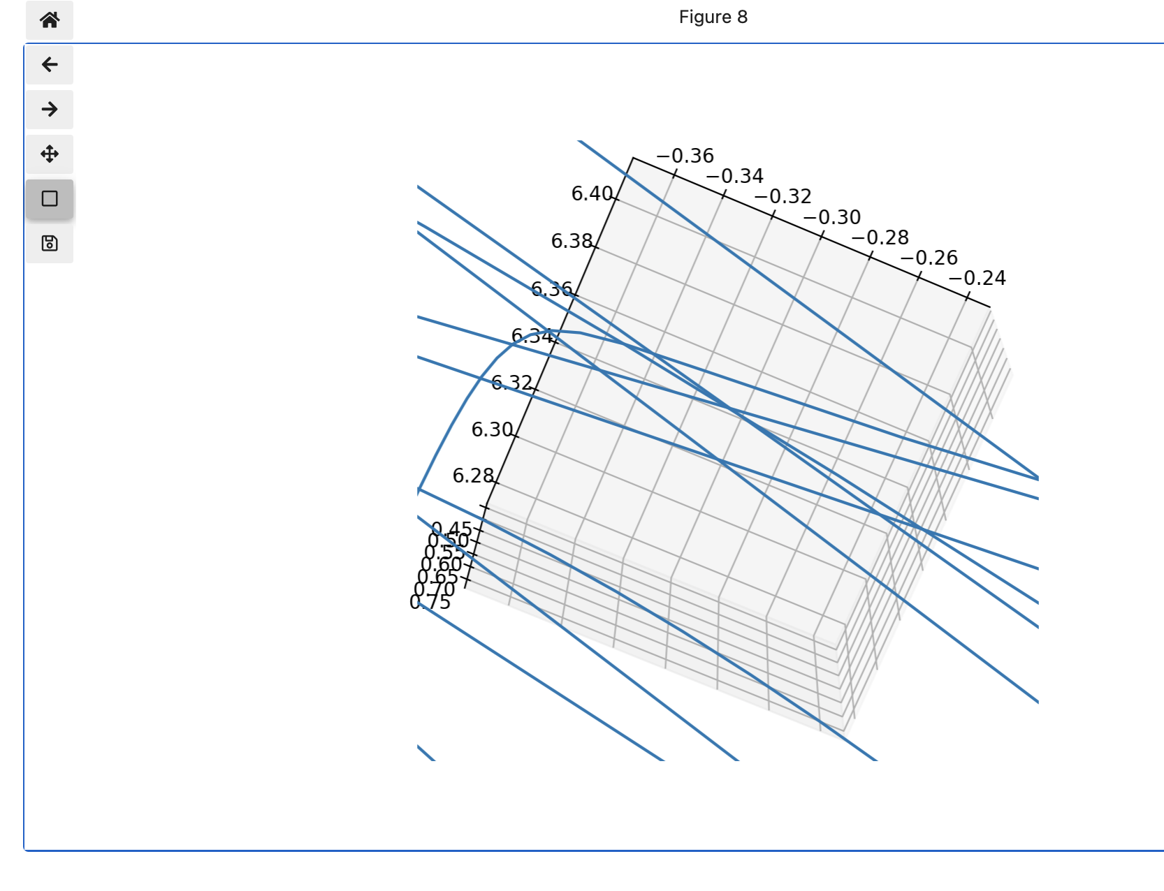
from mpl_toolkits.mplot3d import axes3d

fig = plt.figure()
ax = fig.add_subplot(111, projection='3d')

# Grab some test data.
X, Y, Z = axes3d.get_test_data(0.05)

# Plot a basic wireframe.
ax.plot_wireframe(X, Y, Z, rstride=10, cstride=10)

plt.show()